How to Show that Your Model is Better: A Basic Guide to Statistical Hypothesis Testing

Do you need help determining which machine learning model is superior? This post presents a step-by-step guide using basic statistical techniques and a real case study! 🤖📈 #AIOrthoPraxy #MachineLearning #Statistics #DataScience

When employing Machine Learning to address problems, our choice of a model plays a crucial role. Evaluating models can be straightforward when performance disparities are substantial, for example, when comparing two large-language models (LLMS) on a masked language modeling (MLM) task with 71.01 and 28.56 perplexity, respectively. However, if differences among models are minute, making a solid analysis to discern if one model is genuinely superior to others can prove challenging.

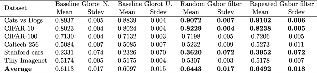
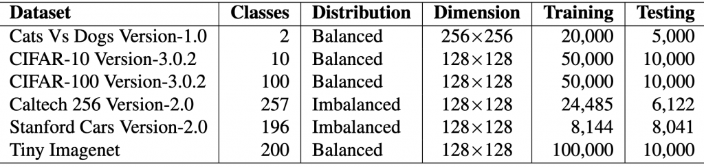
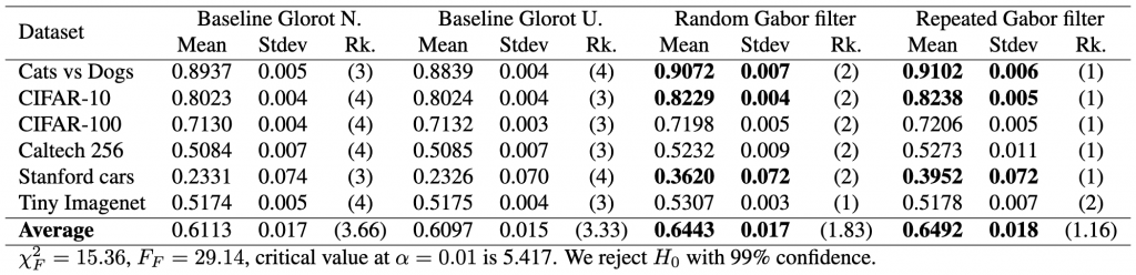
This tutorial aims to present a step-by-step guide to determine if one model is superior to another. Our approach relies on basic statistical techniques and real datasets. Our study compares four models on six datasets using one metric, standard accuracy. Alternatively, other contexts may use different numbers of models, metrics, or datasets. We will work with the tables below that show the properties of the datasets and the performance of two baseline models and two of our proposed models, for which we hope to show that they are better, which would be our hypothesis to be tested.

Summary of performance measured with standard accuracy

Summary of the main properties of the datasets considered in this tutorial.

One of the primary purposes of statistics is hypothesis testing. Statistical inference involves taking a sample from a population and determining how well the sample represents the population. In hypothesis testing, we formulate a null hypothesis, $H_0$ , and an alternative hypothesis, $H_A$ , based on the problem (comparing models). Both hypotheses must be concise, mutually exclusive, and exhaustive. For example, we could say that our null hypothesis is that the models perform equally, and the alternative could mean that the models perform differently.

Why is the ANOVA test not a good alternative?

The ANOVA (Analysis of Variance) test is a parametric test that compares the means of multiple groups. In our case, we have four models to compare with six datasets. The null hypothesis for ANOVA is that all the means are equal, and the alternative hypothesis is that at least one of the means is different. If the $p-$ value of the ANOVA test is less than the significance level (usually 0.05), we reject the null hypothesis and conclude that at least one of the means is different, i.e., at least one model performs differently than the others. However, ANOVA may not always be the best choice for comparing the performance of different models.

One reason for this is that ANOVA assumes that the data follows a normal distribution, which may not always be the case for real-world data. Additionally, ANOVA does not take into account the difficulty of classifying certain data points. For example, in a dataset with a single numerical feature and binary labels, all models may achieve 100% accuracy on the training data. However, if the test set contains some mislabeled points, the models may perform differently. In this scenario, ANOVA would not be appropriate because it does not account for the difficulty of classifying certain data points.

Another issue with ANOVA is that it assumes that the variances of the groups being compared are equal. This assumption may not hold for datasets with different levels of noise or variability. In such cases, alternative statistical tests like the Friedman test or the Nemenyi test may be more appropriate.

Friedman test

The Friedman test is a non-parametric test that compares multiple models. In our example, we want to compare the performance of $k=4$ different models, i.e., two baseline models, Gabor randomized, and Gabor repeated, on $N=6$ datasets. First, the test calculates the average rank of each model’s performance on each dataset, with the best-performing model receiving a rank of 1. The Friedman test then tests the null hypothesis, $H_0$ , that all models are equally effective and their average ranks should be equal. The test statistic is calculated as follows:

(1) $\begin{equation*} \chi_{F}^{2}=\frac{12 N}{k(k+1)}\left[\sum_{j=1}^{k} R_{j}^{2}-\frac{k(k+1)^{2}}{4}\right] \end{equation*}$

where $R$ is the average ranking of each model.

The test result can be used to determine whether there is a statistically significant difference between the performance of the models by making sure that $\chi_{F}^{2}$ is not less than the critical value for the $F$ distribution for a particular confidence value $\alpha$ . However, since $\chi_{F}^{2}$ could be too conservative, we also calculate the $F_F$ statistic as follows:

(2) $\begin{equation*} F_{F}=\frac{(N-1) \chi_{F}^{2}}{N(k-1)-\chi_{F}^{2}}. \end{equation*}$

Based on the critical value, $F_{F}$ , and $\chi_{F}^{2}$ , we evaluate $H_0$ ; once the null hypothesis is rejected, we apply a posthoc test. For this, we use the Nemenyi test to establish whether models differ significantly in their performance.

We will start the process of getting this test done by ranking the data. First, we can load the data and verify it with respect to the table shown earlier.

import pandas as pd
import numpy as np

data = [[0.8937, 0.8839, 0.9072, 0.9102],
        [0.8023, 0.8024, 0.8229, 0.8238],
        [0.7130, 0.7132, 0.7198, 0.7206],
        [0.5084, 0.5085, 0.5232, 0.5273],
        [0.2331, 0.2326, 0.3620, 0.3952],
        [0.5174, 0.5175, 0.5307, 0.5178]]

model_names = ['Glorot N.', 'Glorot U.', 'Random G.', 'Repeated G.']

df = pd.DataFrame(data, columns=model_names)

print(df.describe())  #<- use averages to verify if matches table

Output:

       Glorot N.  Glorot U.  Random G.  Repeated G.
count   6.000000   6.000000   6.000000     6.000000
mean    0.611317   0.609683   0.644300     0.649150
std     0.240422   0.238318   0.206871     0.200173
min     0.233100   0.232600   0.362000     0.395200
25%     0.510650   0.510750   0.525075     0.520175
50%     0.615200   0.615350   0.625250     0.623950
75%     0.779975   0.780100   0.797125     0.798000
max     0.893700   0.883900   0.907200     0.910200

Next, we rank the models and get their averages like so:

data = df.rank(1, method='average', ascending=False)
print(data)
print(data.describe())

Output:

   Glorot N.  Glorot U.  Random G.  Repeated G.
0        3.0        4.0        2.0          1.0
1        4.0        3.0        2.0          1.0
2        4.0        3.0        2.0          1.0
3        4.0        3.0        2.0          1.0
4        3.0        4.0        2.0          1.0
5        4.0        3.0        1.0          2.0

       Glorot N.  Glorot U.  Random G.  Repeated G.
count   6.000000   6.000000   6.000000     6.000000
mean    3.666667   3.333333   1.833333     1.166667
std     0.516398   0.516398   0.408248     0.408248
min     3.000000   3.000000   1.000000     1.000000
25%     3.250000   3.000000   2.000000     1.000000
50%     4.000000   3.000000   2.000000     1.000000
75%     4.000000   3.750000   2.000000     1.000000
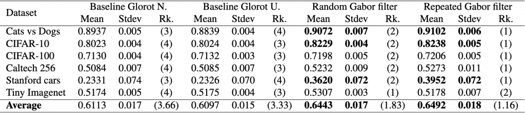
max     4.000000   4.000000   2.000000     2.000000

With this information, we can expand our initial results table to show the rankings by dataset and the average rankings across all datasets for each model.

Now that we have the rankings, we can proceed with the statistical analysis and do the following:

(3) $\begin{align*} \chi_{F}^{2}&=\frac{12 \cdot 6}{4 \cdot 5}\left[\left(3.66^2+3.33^2+1.83^2+1.16^2\right)-\frac{4 \cdot 5^2}{4}\right] \nonumber \\ &=15.364 \nonumber \end{align*}$

(4) $\begin{equation*} F_{F}=\frac{5 \cdot 15.364}{6 \cdot 3-15.364}=29.143 \nonumber \end{equation*}$

The critical value at $\alpha=0.01$ is 5.417. Thus, because the critical value is below our statistics obtained, we reject $H_0$ with 99% confidence.

The critical value can be obtained from any table that has the F distribution. In the table the degrees of freedom across columns (denoted as $df_1$ ) is $k-1$ , that is the number of models minus one; the degrees of freedom across rows (denoted as $df_2$ ) is $(k-1)\times(N-1)$ , that is, the number of models minus one, times the number of datasets minus one. In our case this is $df_1=3$ and $df_2=15$ .

Nemenyi Test

The Nemenyi test is a post-hoc test that compares multiple models after a significant result from Friedman’s test. The null hypothesis for Nemenyi is that there is no difference between any two models, and the alternative hypothesis is that at least one pair of models is different.

The formula for Nemenyi is as follows:

$CD = q_{\alpha} \sqrt{\frac{k(k+1)}{6N}}$

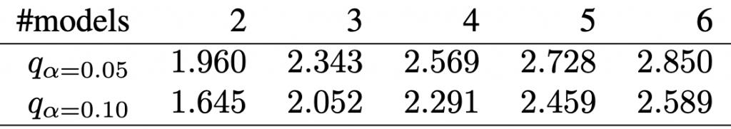
where $q_{\alpha}$ is the critical difference of the Studentized range distribution at the chosen significance level and $k$ is the number of groups. The $q_{\alpha}$ value can be obtained from the following table:

Critical values for the Nemenyi test, which is conducted following the Friedman test, with two-tailed results.

Thus, for our particular case study, the critical differences are:

(5) $\begin{equation*} CD_{\alpha=0.05}=2.569 \sqrt{\frac{4 \cdot 5}{6 \cdot 6}} = 1.915 \nonumber \end{equation*}$

(6) $\begin{equation*} CD_{\alpha=0.10}=2.291 \sqrt{\frac{4 \cdot 5}{6 \cdot 6}} = 1.708 \nonumber \end{equation*}$

Since the difference in rank between the randomized Gabor and baseline Glorot normal is 1.83 and is less than the $CD_{\alpha=0.10}=1.708$ , we conclude Gabor is better. Similarly, since the difference in rank between the fixed Gabor and baseline Glorot uniform is 2.17 and is less than the $CD_{\alpha=0.05}=1.915$ , we conclude that Gabor is better. Yes, there is sufficient statistical evidence to show that our model is better with high confidence.

Things we would like to see in papers

First of all, it would be nice to have a complete table that includes the results of the statistical tests as part of the caption or as a footnote, like this:

Second of all, graphics always help! A simple and visually appealing diagram is a powerful way to represent post hoc test results when comparing multiple classifiers. The figure below, which illustrates the data analysis from the table above, displays the average ranks of methods along the top line of the diagram. To facilitate interpretation, the axis is oriented so that the best ranks appear on the right side, which enables us to perceive the methods on the right as superior.

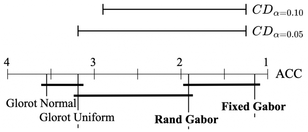
Comparison of all models against each other with the Nemenyi test. Models not significantly different at α = 0.10 or α = 0.05 are connected.

When comparing all the algorithms against each other, the groups of algorithms that are not significantly different are connected with a bold solid line. Such an approach clearly highlights the most effective models while also providing a robust analysis of the differences between models. Additionally, the critical difference is shown above the graph, further enhancing the visualization of the analysis results. Overall, this simple yet powerful diagrammatic approach provides a clear and concise representation of the performance of multiple classifiers, enabling more informed decision-making in selecting the best-performing model.

Main Sources

The statistical tests are based on this paper:

Demšar, Janez. “Statistical comparisons of classifiers over multiple data sets.” The Journal of Machine learning research 7 (2006): 1-30.

The case study is based on the following research:

Rai, Mehang. “On the Performance of Convolutional Neural Networks Initialized with Gabor Filters.” Thesis, Baylor University, 2021.

Why is the ANOVA test not a good alternative?

Friedman test

Nemenyi Test

Things we would like to see in papers

Main Sources

Share this:

Leave a Reply Cancel reply