
As we gather around the table this Thanksgiving, it’s the perfect time to reflect on and express gratitude for the remarkable strides made in machine learning (ML) over recent years. These technical innovations have advanced the field and paved the way for countless applications that enhance our daily lives. Let’s check out some of the most influential ML architectures and algorithms for which we are thankful as a community.
1. The Transformer Architecture
Vaswani et al., 2017
We are grateful for the Transformer architecture, which revolutionized sequence modeling by introducing a novel attention mechanism, eliminating the reliance on recurrent neural networks (RNNs) for handling sequential data.
Key Components:
- Self-Attention Mechanism: Computes representations of the input sequence by relating different positions via attention weights.

- Multi-Head Attention: Allows the model to focus on different positions by projecting queries, keys, and values multiple times with different linear projections.
 where each head is computed as:
- Positional Encoding: Adds information about the position of tokens in the sequence since the model lacks recurrence.

Significance: Enabled parallelization in sequence processing, leading to significant speed-ups and improved performance in tasks like machine translation and language modeling.
2. Bidirectional Encoder Representations from Transformers (BERT)
Devlin et al., 2018
We are thankful for BERT, which introduced a method for pre-training deep bidirectional representations by jointly conditioning on both left and right contexts in all layers.
Key Concepts:
- Masked Language Modeling (MLM): Randomly masks tokens in the input and predicts them using the surrounding context. Loss Function:
 where
where  is the set of masked positions.
 - Next Sentence Prediction (NSP): Predicts whether a given pair of sentences follows sequentially in the original text.
Significance: Achieved state-of-the-art results on a wide range of NLP tasks via fine-tuning, demonstrating the power of large-scale pre-training.
3. Generative Pre-trained Transformers (GPT) Series
Radford et al., 2018-2020
We express gratitude for the GPT series, which leverages unsupervised pre-training on large corpora to generate human-like text.
Key Features:
- Unidirectional Language Modeling: Predicts the next token
 given previous tokens
  . Objective Function:
- Decoder-Only Transformer Architecture: Utilizes masked self-attention to prevent the model from attending to future tokens.
Significance: Demonstrated the capability of large language models to perform few-shot learning, adapting to new tasks with minimal task-specific data.
4. Variational Autoencoders (VAEs)
Kingma and Welling, 2013
We appreciate VAEs for introducing a probabilistic approach to autoencoders, enabling generative modeling of complex data distributions.
Key Components:
- Encoder Network: Learns an approximate posterior
 .
. - Decoder Network: Reconstructs the input from latent variables
 , modeling
  .
.
Objective Function (Evidence Lower Bound – ELBO): ![\mathcal{L}(\theta, \phi; x) = -\text{KL}(q_{\phi}(z|x) \| p_{\theta}(z)) + \mathbb{E}_{q_{\phi}(z|x)}[\log p_{\theta}(x|z)]](https://baylor.ai/wp-content/ql-cache/quicklatex.com-92d0f4d5005687fea92672cd46704072_l3.png "Rendered by QuickLaTeX.com") where
where  is typically a standard normal prior
  .
.
Significance: Provided a framework for unsupervised learning of latent representations and generative modeling.
5. Generative Adversarial Networks (GANs)
Goodfellow et al., 2014
We are thankful for GANs, which consist of two neural networks—a generator  and a critic
  —competing in a minimax game.
Objective Function: ![\min_G \max_D V(D, G) = \mathbb{E}_{x \sim p_{\text{data}}}[\log D(x)] + \mathbb{E}_{z \sim p_z}[\log(1 - D(G(z)))]](https://baylor.ai/wp-content/ql-cache/quicklatex.com-f4c6097b521f4afe7b8923e542639fb8_l3.png "Rendered by QuickLaTeX.com") where
where  is the data distribution and
  is the prior over the latent space.
Significance: Enabled the generation of highly realistic synthetic data, impacting image synthesis, data augmentation, and more.
6. Deep Reinforcement Learning
Mnih et al., 2015; Silver et al., 2016
We give thanks for the combination of deep learning with reinforcement learning, leading to agents capable of performing complex tasks.
Key Algorithms:
- Deep Q-Networks (DQN): Approximate the action-value function
 using neural networks. Bellman Equation:
  where
where  are the parameters of a target network.
 - Policy Gradient Methods: Optimize the policy
 directly. REINFORCE Algorithm Objective:
 ![\nabla_{\theta} J(\theta) = \mathbb{E}_{\pi_{\theta}} \left[ \nabla_{\theta} \log \pi_{\theta}(a|s) R \right]](https://baylor.ai/wp-content/ql-cache/quicklatex.com-e53cb7a1cae29f8595a1b83926e92a7f_l3.png "Rendered by QuickLaTeX.com") where
where  is the cumulative reward.
Significance: Achieved human-level performance in games like Atari and Go, advancing AI in decision-making tasks.
7. Normalization Techniques
We are grateful for normalization techniques that have improved training stability and performance of deep networks.
- Batch Normalization (Ioffe and Szegedy, 2015) Formula:
 where
where  and
and  are the batch mean and variance.
 - Layer Normalization (Ba et al., 2016) Formula:
 where
where  and
and  are computed over the features of a single sample.
Significance: Mitigated internal covariate shift, enabling faster and more reliable training.
8. Attention Mechanisms in Neural Networks
Bahdanau et al., 2014; Luong et al., 2015
We appreciate attention mechanisms for allowing models to focus on specific parts of the input when generating each output element.
Key Concepts:
- Alignment Scores: Compute the relevance between encoder hidden states
 and decoder state
  . Common Score Functions:
- Dot-product:

- Additive (Bahdanau attention):
![\text{score}(h, s) = v_a^\top \tanh(W_a [h; s])](https://baylor.ai/wp-content/ql-cache/quicklatex.com-c1390492617640d0676cb7559ef2b7e6_l3.png "Rendered by QuickLaTeX.com")
- Dot-product:
- Context Vector:
 where the attention weights
  are computed as:
Significance: Enhanced performance in sequence-to-sequence tasks by allowing models to utilize information from all input positions.
9. Graph Neural Networks (GNNs)
Scarselli et al., 2009; Kipf and Welling, 2016
We are thankful for GNNs, which extend neural networks to graph-structured data, enabling the modeling of relational information.
Message Passing Framework:
- Node Representation Update:
 where:
 is the representation of node
  at layer
  .
. is the set of neighbors of node .
 and
and  are learnable weight matrices.
 is a nonlinear activation function.
- Graph Convolutional Networks (GCNs):
 where:
 is the adjacency matrix with added self-loops.
 is the degree matrix of
  .
.
Significance: Enabled advancements in social network analysis, molecular chemistry, and recommendation systems.
10. Self-Supervised Learning and Contrastive Learning
He et al., 2020; Chen et al., 2020
We are grateful for self-supervised learning techniques that leverage unlabeled data by creating surrogate tasks.
Contrastive Learning Objective:
- InfoNCE Loss:
![\mathcal{L}_{i,j} = -\log \frac{\exp(\text{sim}(z_i, z_j)/\tau)}{\sum_{k=1}^{2N} \textbf{1}_{[k \neq i]} \exp(\text{sim}(z_i, z_k)/\tau)}](https://baylor.ai/wp-content/ql-cache/quicklatex.com-6a9932a8dfe6978287a7781d76d979c1_l3.png "Rendered by QuickLaTeX.com") where:
where:
 and
and  are representations of two augmented views of the same sample.
 is the cosine similarity.
 is a temperature parameter.
![\textbf{1}_{[k \neq i]}](https://baylor.ai/wp-content/ql-cache/quicklatex.com-bf75515a28c2f067b99872a895694ed8_l3.png "Rendered by QuickLaTeX.com") is an indicator function equal to 1 when
is an indicator function equal to 1 when  .
.
Significance: Improved representation learning, leading to state-of-the-art results in computer vision tasks without requiring labeled data.
11. Differential Privacy in Machine Learning
Abadi et al., 2016
We give thanks for techniques that allow training models while preserving the privacy of individual data points.
Differential Privacy Guarantee:
- Definition: A randomized algorithm
 provides
  -differential privacy if for all datasets and
  differing on one element, and all measurable subsets
  :
: ![P[\mathcal{A}(D) \in S] \leq e^\epsilon P[\mathcal{A}(D') \in S] + \delta](https://baylor.ai/wp-content/ql-cache/quicklatex.com-fc3bfc99a2d0988d512d785abdbbe75c_l3.png "Rendered by QuickLaTeX.com")
- Noise Addition: Applies calibrated noise to gradients during training to ensure privacy.
Significance: Enabled the deployment of machine learning models in privacy-sensitive applications.
12. Federated Learning
McMahan et al., 2017
We are thankful for federated learning, which allows training models across multiple decentralized devices while keeping data localized.
Federated Averaging Algorithm:
- Local Update: Each client updates model parameters
 using local data
  :
: 
- Global Aggregation: The server aggregates updates:
 where:
 is the number of samples at client .
 is the total number of samples across all clients.
Significance: Addressed privacy concerns and bandwidth limitations in distributed systems.
13. Neural Architecture Search (NAS)
Zoph and Le, 2016
We appreciate NAS for automating the design of neural network architectures using optimization algorithms.
Approaches:
- Reinforcement Learning-Based NAS: Uses an RNN controller to generate architectures, trained to maximize expected validation accuracy.
- Differentiable NAS (DARTS): Models the architecture search space as continuous, enabling gradient-based optimization. Objective Function:
 where
where  is obtained by:
Significance: Reduced human effort in designing architectures, leading to efficient and high-performing models.
14. Optimizer Advancements (Adam, AdaBound, RAdam)
We are thankful for advancements in optimization algorithms that improved training efficiency.
- Adam Optimizer(Kingma and Ba, 2014)
Update Rules: ,
,  ,
,  ,
,  ,
, 
where: is the gradient at time step
  .
. and
and  are hyperparameters controlling the exponential decay rates.
 is the learning rate.
 is a small constant to prevent division by zero.
Significance: Improved optimization efficiency and convergence in training deep neural networks.
15. Diffusion Models for Generative Modeling
Ho et al., 2020; Song et al., 2020
We give thanks for diffusion models, which are generative models that learn data distributions by reversing a diffusion (noising) process.
Key Concepts:
- Forward Diffusion Process: Gradually adds Gaussian noise to data over
 timesteps.
Noising Schedule:
- Reverse Process: Learns to denoise from
 back to
  .
.
Objective Function:![\mathcal{L}_{\text{simple}} = \mathbb{E}_{t, x_0, \epsilon} \left[ \| \epsilon - \epsilon_\theta(x_t, t) \|^2 \right]](https://baylor.ai/wp-content/ql-cache/quicklatex.com-ef4693d6547fa2ffa2c1970ed721c48e_l3.png "Rendered by QuickLaTeX.com") where:
where:
- is the noise added to the data.
 is the model’s prediction of the noise at timestep .
Significance: Achieved state-of-the-art results in image generation, rivaling GANs without their training instability.
Give Thanks…
This Thanksgiving, let’s celebrate and express our gratitude for these groundbreaking contributions to machine learning. These technical advancements have not only pushed the boundaries of what’s possible but have also laid the foundation for future innovations that will continue to shape our world.
May we continue to build upon these foundations and contribute to the growing field of machine learning.
References
- Vaswani, A., Shazeer, N., Parmar, N., Uszkoreit, J., Jones, L., Gomez, A. N., Kaiser, Ł., & Polosukhin, I. (2017). Attention is All You Need. Advances in Neural Information Processing Systems. arXiv:1706.03762
- Devlin, J., Chang, M. W., Lee, K., & Toutanova, K. (2018). BERT: Pre-training of Deep Bidirectional Transformers for Language Understanding. arXiv:1810.04805
- Radford, A., Narasimhan, K., Salimans, T., & Sutskever, I. (2018). Improving Language Understanding by Generative Pre-training. OpenAI Blog.
- Kingma, D. P., & Welling, M. (2013). Auto-Encoding Variational Bayes. arXiv:1312.6114
- Goodfellow, I., Pouget-Abadie, J., Mirza, M., Xu, B., Warde-Farley, D., Ozair, S., Courville, A., & Bengio, Y. (2014). Generative Adversarial Nets. Advances in Neural Information Processing Systems.
- Mnih, V., Kavukcuoglu, K., Silver, D., Rusu, A. A., Veness, J., Bellemare, M. G., Graves, A., Riedmiller, M., Fidjeland, A. K., Ostrovski, G., Petersen, S., Beattie, C., Sadik, A., Antonoglou, I., King, H., Kumaran, D., Wierstra, D., Legg, S., & Hassabis, D. (2015). Human-level Control through Deep Reinforcement Learning. Nature.
- Ioffe, S., & Szegedy, C. (2015). Batch Normalization: Accelerating Deep Network Training by Reducing Internal Covariate Shift. International Conference on Machine Learning (ICML).
- Ba, J. L., Kiros, J. R., & Hinton, G. E. (2016). Layer Normalization. arXiv:1607.06450
- Bahdanau, D., Cho, K., & Bengio, Y. (2014). Neural Machine Translation by Jointly Learning to Align and Translate. arXiv:1409.0473
- Kipf, T. N., & Welling, M. (2016). Semi-Supervised Classification with Graph Convolutional Networks. arXiv:1609.02907
- He, K., Fan, H., Wu, Y., Xie, S., & Girshick, R. (2020). Momentum Contrast for Unsupervised Visual Representation Learning. arXiv:1911.05722
- Abadi, M., Chu, A., Goodfellow, I., McMahan, H. B., Mironov, I., Talwar, K., & Zhang, L. (2016). Deep Learning with Differential Privacy. ACM SIGSAC Conference on Computer and Communications Security.
- McMahan, B., Moore, E., Ramage, D., Hampson, S., & y Arcas, B. A. (2017). Communication-Efficient Learning of Deep Networks from Decentralized Data. arXiv:1602.05629
- Zoph, B., & Le, Q. V. (2016). Neural Architecture Search with Reinforcement Learning. arXiv:1611.01578
- Kingma, D. P., & Ba, J. (2014). Adam: A Method for Stochastic Optimization. arXiv:1412.6980
- Ho, J., Jain, A., & Abbeel, P. (2020). Denoising Diffusion Probabilistic Models. arXiv:2006.11239
![\[\min_{\mathcal{O}}\mathbb{E}[ \left | \langle{\psi}| \mathcal{O} |{\psi} \rangle - \langle{\psi} | \mathcal{O}_n |{\psi} \rangle ]\]](https://baylor.ai/wp-content/ql-cache/quicklatex.com-3cfa5f0083acaa8744a5fc03feba12bf_l3.png "Rendered by QuickLaTeX.com")
 is a Pauli-Z observable, and
  is an observable we are trying to learn. The expectation value is computed before and after noise is introduced. The goal is to find an observable that minimizes this difference, effectively learning a robust observable.
 . The expectation values of the observable
  on the depolarized Bell state as a function of the depolarization rate
  are plotted in the following figure.
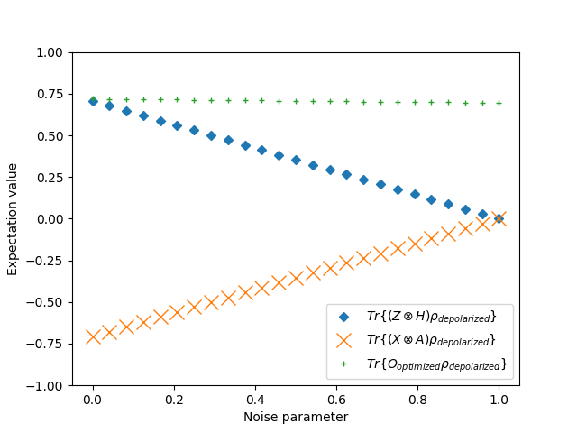
 is the Pauli-Z matrix,
  is the Pauli-X matrix,
  is the Hadamard gate,
  is an arbitrary observable, and


 , and an alternative hypothesis,
  , based on the problem (comparing models). Both hypotheses must be concise, mutually exclusive, and exhaustive. For example, we could say that our null hypothesis is that the models perform equally, and the alternative could mean that the models perform differently.
 value of the ANOVA test is less than the significance level (usually 0.05), we reject the null hypothesis and conclude that at least one of the means is different, i.e., at least one model performs differently than the others. However, ANOVA may not always be the best choice for comparing the performance of different models.
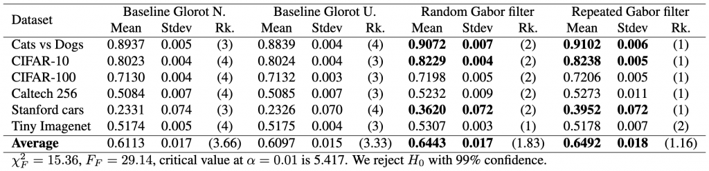
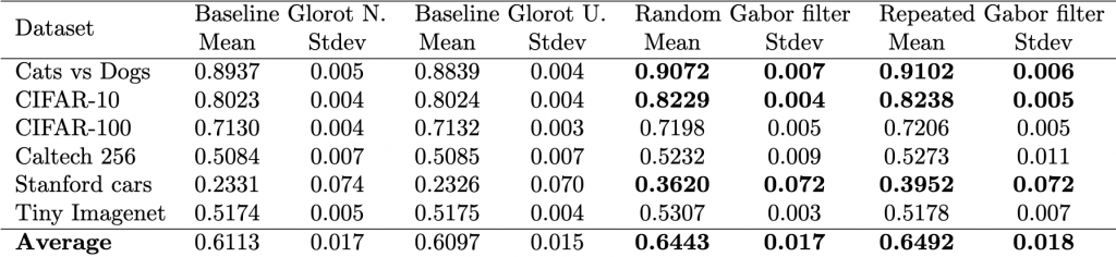
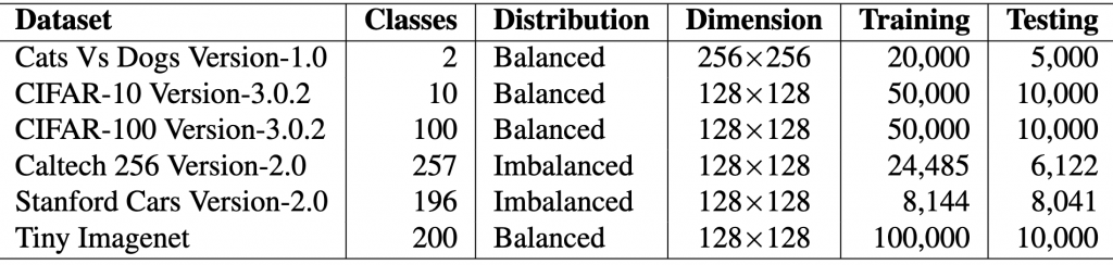
 different models, i.e., two baseline models, Gabor randomized, and Gabor repeated, on
  datasets. First, the test calculates the average rank of each model’s performance on each dataset, with the best-performing model receiving a rank of 1. The Friedman test then tests the null hypothesis,
 ![\begin{equation*} \chi_{F}^{2}=\frac{12 N}{k(k+1)}\left[\sum_{j=1}^{k} R_{j}^{2}-\frac{k(k+1)^{2}}{4}\right] \end{equation*}](https://baylor.ai/wp-content/ql-cache/quicklatex.com-e2518869970055a72a2524df63957827_l3.png "Rendered by QuickLaTeX.com")
 is not less than the critical value for the
  distribution for a particular confidence value
  . However, since
  statistic as follows:

 , and
, and 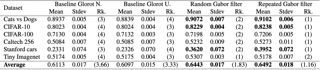
![\begin{align*} \chi_{F}^{2}&=\frac{12 \cdot 6}{4 \cdot 5}\left[\left(3.66^2+3.33^2+1.83^2+1.16^2\right)-\frac{4 \cdot 5^2}{4}\right] \nonumber \\ &=15.364 \nonumber \end{align*}](https://baylor.ai/wp-content/ql-cache/quicklatex.com-b7fd261f286621cdf8d57b028898841d_l3.png "Rendered by QuickLaTeX.com")

 is 5.417. Thus, because the critical value is below our statistics obtained, we reject
  ) is
) is  , that is the number of models minus one; the degrees of freedom across rows (denoted as
  ) is
) is  , that is, the number of models minus one, times the number of datasets minus one. In our case this is
  and
and  .
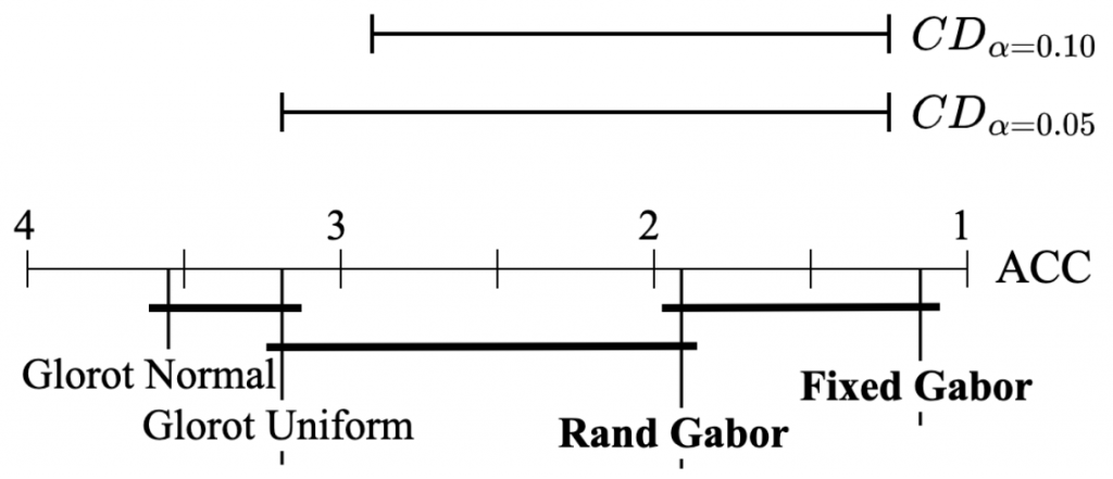
.![\[CD = q_{\alpha} \sqrt{\frac{k(k+1)}{6N}}\]](https://baylor.ai/wp-content/ql-cache/quicklatex.com-31ddfa7633974f9a4c569740f85c93b8_l3.png "Rendered by QuickLaTeX.com")
 is the critical difference of the Studentized range distribution at the chosen significance level and
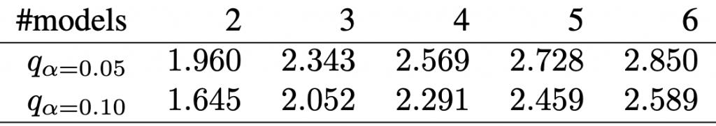


 , we conclude Gabor is better. Similarly, since the difference in rank between the fixed Gabor and baseline Glorot uniform is 2.17 and is less than the
  , we conclude that Gabor is better. Yes, there is sufficient statistical evidence to show that our model is better with high confidence.